Investors currently face the challenge of having little experience and no recent data to guide the repositioning of their portfolios in the face of heighted inflation risk. We provide some insight.
AUGUST 2021
Over the past three decades, a sustained surge in inflation has been absent in developed markets. As a result, investors faced the challenge of having little experience and no recent data to guide the repositioning of their portfolios in the face of heighted inflation risk. We provide some insight by analysing both passive and active strategies across a variety of asset classes for the US, UK and Japan over the past 95 years. Unexpected inflation is bad news for traditional assets, such as bonds and equities, with local inflation having the greatest effect. Commodities have positive returns during inflation surges, but there is considerable variation within the commodity complex. Among the active strategies, we find that trend-following provides the most reliable protection during important inflation shocks. Active equity factor strategies also provide some degree of hedging ability. We also provide analysis of alternative asset classes such as fine art and discuss the economic rationale for including cryptocurrencies as part of a strategy to protect against inflation.
Link para o artigo original : https://www.man.com/maninstitute/best-strategies-for-inflationary-times
Man Group is a global, technology-empowered active investment management firm focused on delivering alpha and portfolio solutions for clients. Headquartered in London, we manage $127 billion* and operate across multiple offices globally.
We invest across a diverse range of strategies and asset classes, with a mix of long only and alternative strategies run on a discretionary and quantitative basis, across liquid and private markets. Our investment teams work within Man Group’s single operating platform, enabling them to invest with a high degree of empowerment while benefiting from the collaboration, strength and resources of the entire firm. Our platform is underpinned by advanced technology, supporting our investment teams at every stage of their process, including alpha generation, portfolio management, trade execution and risk management.
Our clients and the millions of retirees and savers they represent are at the heart of everything we do. We form deep and long-lasting relationships and create tailored solutions to help meet their
unique needs. We recognise that responsible investing is intrinsically linked to our fiduciary duty to our clients, and we integrate this approach broadly across the firm.
We are committed to creating a diverse and inclusive workplace where difference is celebrated and everyone has an equal opportunity to thrive, as well as giving back and contributing positively to our communities. For more information about Man Group’s global charitable efforts, and our diversity and inclusion initiatives, please visit: https://www.man.com/corporate-responsibility
Man Group plc is listed on the London Stock Exchange under the ticker EMG.LN and is a constituent of the FTSE 250 Index. Further information can be found at www.man.com
*As at 31 March 2021. All investment management and advisory services are offered through the investment “engines” of Man AHL, Man Numeric, Man GLG, Man Solutions / FRM and Man GPM.

Henry Neville is an associate director at Man Group. He has been at Man Group since
2016.
Previously, he was an equity analyst at Walter Scott & Partners, a subsidiary of BNY Mellon,
and a graduate analyst at Hoares Bank.
He studied History at St. Andrew’s University and is a CFA charterholder.

Teun Draaisma is the joint lead Portfolio Manager within Man Group’s multi-asset offering. He
joined Man Group in May 2018 from BlackRock, where he was global equity strategist since
2012, focusing on portfolio management and asset allocation.
Prior to this, he was European equity strategist at Morgan Stanley from 1997 to 2010, where
he ran the European Equity Strategy team. He has also been a portfolio manager at TT
International.
Teun holds a master’s degree in Econometrics from Erasmus University Rotterdam.

Ben Funnell is the joint lead Portfolio Manager within Man Group’s multi-asset offering.
Previously, he was a lead portfolio manager and chief equity strategist at Man GLG.
Prior to joining Man GLG in 2005, he spent 11 years at Morgan Stanley, the last nine
of those years on the European Equity Strategy team, which he co-headed in his final
three years at the firm.
He was educated in modern languages at Durham University, UK.

Campbell R. Harvey has been an Investment Strategy Advisor to Man Group since 2005.
He is a Professor of Finance at Duke University and Research Associate at the National
Bureau of Economic Research in Cambridge, Massachusetts. He served as Editor of
The Journal of Finance from 2006 to 2012 and as the 2016 President of the American
Finance Association. For the last five years, Campbell has taught a course called Innovation
and Cryptoventures that focuses on the mechanics and applications of blockchain
technology. He holds a PhD in Finance from the University of Chicago.

Otto Van Hemert is Director of Core Strategies and a member of Man AHL’s management
and investment committees.
He was previously Head of Macro Research at Man AHL. Prior to joining Man AHL in
2015, Otto ran a systematic global macro fund at IMC for more than three years. Before
that, he headed Fixed Income Arbitrage, Credit, and Volatility strategies at AQR, and was
on the Finance Faculty at the New York University Stern School of Business, where he
published papers in leading academic finance journals.
Otto holds a PhD in Economics and Masters Degrees in Mathematics and Economics.
The Best Strategies for
Inflationary Times
Henry Neville, Teun Draaisma, Ben Funnell, Campbell R. Harvey,
and Otto Van Hemert
KEY FINDINGS
- The authors examine a range of passive and active strategies using a century of data
in the United States, the United Kingdom, and Japan and find that passive equity and
fixed-income strategies fare poorly during inflation surges. - Commodities provide historical inflation protection, as do collectibles such as wine and
fine art. - Active strategies such as trend-following fare well during historical inflation surges, and
equity factor strategies such as quality provide some protection.
ABSTRACT
Over the past three decades, a sustained surge in inflation has been absent in developed
markets. As a result, investors face the challenge of having limited experience and no
recent data to guide the repositioning of their portfolios in the face of heightened inflation
risk. In this article, the authors provide some insight by analyzing both passive and active
strategies across a variety of asset classes for the United States, the United Kingdom,
and Japan over the past 95 years. Unexpected inflation is bad news for traditional assets,
such as bonds and equities, with local inflation having the greatest effect. Commodities
have positive returns during inflation surges, but there is considerable variation within the
commodity complex. Among the active strategies, the authors find that trend-following
provides the most reliable protection during important inflation shocks. Active equity factor
strategies also provide some degree of hedging ability. The authors also provide an analysis
of alternative asset classes such as fine art and discuss the economic rationale for including
cryptocurrencies as part of a strategy to protect against inflation.
TOPICS
Developed markets, financial crises and financial market history, risk management,
portfolio management/multi-asset allocation*
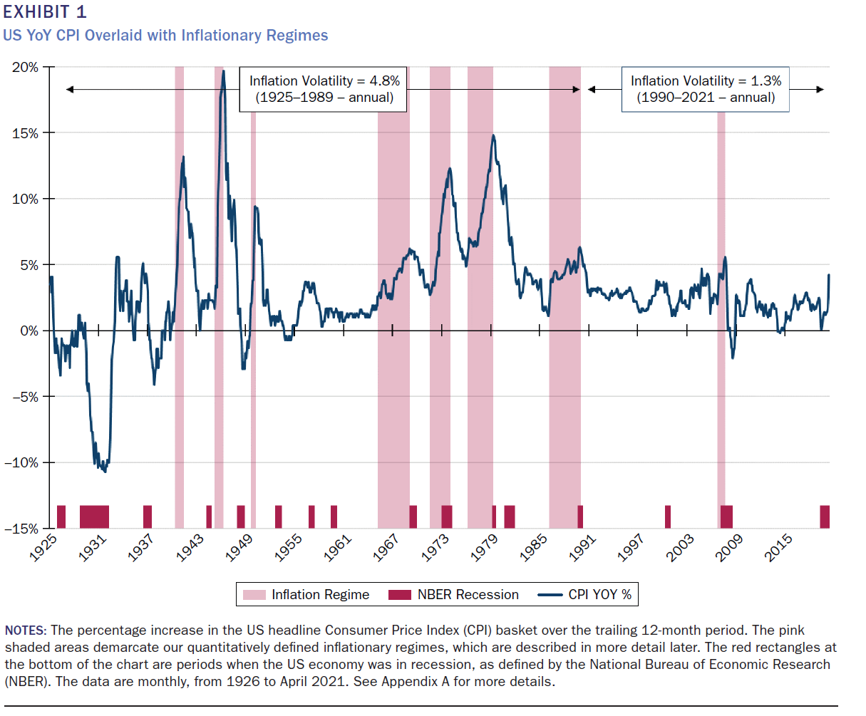
Inflation has not been a serious and persistent economic problem in developed markets for decades. Both monetary and fiscal policy have contributed to economic circumstances that are disinflationary, resulting in lower and less volatile inflation(Exhibit 1). Today, those fearful of an inflation resurgence point to at least two factors that suggest the risk has increased.
First, there has been an unprecedented increase in money creation. The US money supply (M2) has grown by $4.9 trillion, from $15.5 trillion to $20.4 trillion in the 16 months between February 2020 and June 2021. Second, there has been extraordinary fiscal accommodation. The Congressional Budget Offi ce (CBO) estimates a US fiscal deficit of $3.1 trillion in 2020, or 14.9% of gross domestic product (GDP). The CBO forecasts the defi cit will be slightly reduced to $3.0 trillion in 2021, or 13.4% of GDP. In the entire modern history of the United States, there have only been twoinstances of consecutive double-digit deficit years.¹
Rather than predicting when (or if) inflation will increase to disruptive levels, this article seeks to answer a simpler question: What passive and active investments have historically tended to do well (or poorly) in environments of high and rising inflation? The answer to this question may help investors reposition their portfolios so that they are better prepared should current fears prove justified.
We define inflationary regimes as the times when headline, year-over-year (YoY) infl ation is accelerating and when the level moves to 5% or more. We detail the complete formulation of the regime classification later. Based on this defi nition, we identify the eight US inflationary regimes shaded pink in Exhibit 1. We argue that episodes of high and rising inflation rates are mostly due to unexpected inflation, and assets may reprice materially during such regimes. To assemble a critical mass of evidence, we use data from 1926, across three continents.
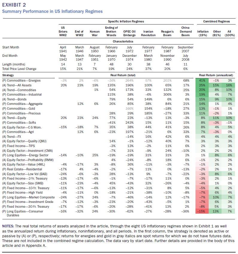
In Exhibit 2, we summarize our main fi ndings for the United States. We rank the various passive and active strategies by the annualized average real returns during the eight inflationary regimes (the pink shaded zones in Exhibit 1). Weak returns are observed for nominal bonds. This is not surprising because rising infl ation is typically associated with rising yields and thus declining bond prices. Perhaps more notable is that equities also perform poorly, compounding the challenge of the 60–40 equity–bond investor. The best historical performance is observed for commodities; in fact, commodities show much higher real returns during rising inflation environments than at other times.
We start our empirical examination by detailing the economic mechanisms that link unexpected inflation to asset returns. Next, we set out to define what we mean by inflationary periods, identifying 34 episodes from 1926 across the United States, the United Kingdom, and Japan. We show that neither equities nor bonds perform well in real terms during inflationary regimes. Equities may be expected to deliver some inflation protection, as a firm’s debt obligations are inflated away, and product prices may be adjusted to inflation. In reality, equities suffer from the less stable economic climate, and costs tend to rise with inflation more than output prices. Moreover, we find that no individual equity sector offers significant protection against high and rising inflation; even the energy sector is only slightly better than flat in real terms. Nominal bonds do not deliver inflation protection, as expected, and performance deteriorates as duration lengthens. Real returns to credit are also negative. Treasury inflation-protected securities (TIPS) are robust when inflation rises, giving them the benefit of generating similar real returns in inflationary and noninflationary regimes, both of which are positive.
We find that traded commodities have historically performed best during high and rising inflation. In aggregate, they have a perfect track record of generating positive real returns during our eight US regimes, averaging an annualized +14% real return. This contrasts with normal periods, when the commodity aggregate returns are in the low single digits. We also evaluate residential real estate and find that although on average it holds its value during inflationary times (real returns are negative but not of significant magnitude), it lags commodities significantly. Collectibles such as art, wine, and stamps are also examined. We find strong real returns during inflationary periods (although still weaker than commodities), but clearly the extent to which these can form a sizeable part of institutional mandates is very limited given liquidity constraints. We also discuss the case for investing in cryptocurrencies such as bitcoin as an inflation hedge.
We also analyze a number of active strategies. We find that cross-sectional stock momentum is the best equity factor during our inflationary regimes, realizing an 8% annual real return versus 4% in normal times. However, as we will argue later, the difference is not statistically significant for this volatile, high-turnover strategy. That said, active equity factors generally hold their own during inflation surges, with quality having a small positive real return and value having a small negative return. We also follow the method of Hamill, Rattray, and Van Hemert (2016) and Harvey, Rattray, and Van Hemert (2021) and construct a time-series momentum (trend) strategy applied to liquid futures and forwards across assets. This trend strategy performs well during inflationary regimes, with the bond and commodity trend doing particularly well. This lines up with our intuition that inflation shocks do not tend to be overnight affairs, but rather prolonged episodes that play to the strength of trend strategies.
Although trend strategies tend to outperform equity factor strategies in high and rising inflationary regimes, we are cognizant that the former have more limited capacity than the latter, a key consideration for many institutional investors. In this context, the modest protection provided by, for example, quality, which averages 3% in inflationary times, may still be useful, especially in comparison with the sharp losses experienced in long-only financial assets.
WHY DOES INFLATION MATTER FOR ASSET PRICES?
Economic Mechanism
There is a deep academic literature that focuses on the economic mechanisms that link unexpected inflation to asset prices.² It is essential to distinguish between temporary and permanent (or longer-lasting) inflation shocks. Asset prices such as equities and bonds are long-lived and are most sensitive to changes in perceptions about longer-term inflation. For example, a month-long disruption of a gas pipeline might cause gasoline prices (and inflation) to temporarily surge, whereas the impact on asset prices would be minimal because market participants would expect prices
to return to normal in the next month. This example highlights two key challenges in conducting research linking inflation shocks to asset prices: separating permanent and temporary shocks and identifying the most relevant inflation horizon.
Treasury bond prices are obviously affected by unexpected inflation. Their current prices reflect an expected real interest rate, an expected rate of inflation, and a risk premium. If there is an unexpected surge in inflation, the expected inflation embedded in the yield increases and the bond price usually falls. If the new level of expected inflation is permanent, bonds with higher durations will be more sensitive than those with shorter durations. Indeed, with bonds we know the exact inflation horizon that is relevant, given the fixed bond maturity. A change in uncertainty about inflation rates may also affect the risk premium.
Equities are more complicated, and there are a number of ways in which increased inflation can affect equity prices. First, higher and more volatile inflation creates more economic uncertainty, thus harming the ability of companies to plan, invest, grow, and engage in longer-term contracts. Moreover, although firms with market power can increase their output prices to mitigate the impact of an inflation surprise, many companies can only partially pass on the increased cost of raw materials. Margins therefore shrink. Second, unexpected inflation may be associated with future economic weakness. Although an overheating may cause companies’ revenues to increase in the short term, if the inflation is followed by economic weakness,³ this will decrease
expected future cash flows. Third, there is a tax implication for companies with high capital expenditures. Given that depreciation is calculated based on the asset’s historical cost (unadjusted for change in the Consumer Price Index [CPI]), the recognized expense will be artificially low in an environment of high and rising inflation, effectively creating an inflation tax. Of course, many companies today rely heavily on intangible capital and are relatively immune to this effect. Fourth, unexpected inflation could serve to increase risk premiums (increase discount rates), thus reducing equity prices. Finally, similar to bond markets, high-duration stocks (particularly growth stocks that promise dividends far in the future) are especially sensitive to increased discount
rates that result from changing perceptions of long-term inflation.
The inflation mechanism for commodities, like bonds, is relatively straightforward. Indeed, commodities are often the source of inflation. However, commodities are also a diverse asset class, and although some move closely with inflation, others do not.
Expected and Unexpected Inflation
Investors seek to hedge unexpected inflation. Indeed, expected inflation is easy to hedge because bond prices already reflect it. Previous research has focused on two types of inflation risk measures. The first is a measure of unexpected inflation (i.e., the realized level of inflation minus the expected inflation, or the actual level at time tminus the forecast for time t made at time t – 1). The expected inflation rate may be derived from professional forecasts or a statistical model. Typically, the change in the rate of inflation is used as a proxy for unexpected inflation. This formulation assumes that the best forecast of the next period’s inflation rate is the current period’s rate. Research has suggested that this simple model is a good approximation compared to other measures of inflation forecasts, such as survey measures (Ang 2014).
However, there are still numerous issues in measuring unexpected inflation. For example, although the measure is straightforward when implemented for one month, one quarter, or even one year, it is not obvious how we should treat longer-horizon inflation. It is unlikely that the term structure of expected inflation is flat. Indeed, per our earlier example, a large monthly inflation shock could be irrelevant for asset prices if market participants believe it will be reversed in the near future. As a result, another approach measures the change in expected inflation. For example, this could be measured as the change in the breakeven inflation (BEI) rate reflected in TIPS and nominal Treasuries. The BEI is the weighted average of inflation expectations over the life of the bond. Changes in the BEI have the advantage of reflecting changes in long-term or permanent inflation expectations. Unfortunately, BEI data are only available from 1997, limiting their usefulness in the analysis of historical inflation surges.
In our research, we will measure how asset returns vary in response to unexpected inflation. This is akin to an inflation beta. We expect bonds and equities to have negative inflation betas, whereas certain commodities will likely have positive betas. However, relatively little is known about the sensitivity of active strategies to unexpected inflation. One of our contributions is to detail the inflation-hedging properties of various equity factor strategies as well as active trend strategies. Of course, inflation betas are measured with noise because our measure of unexpected inflation (change in inflation rate) focuses exclusively on the short term and is unable to separate the temporary and permanent components.
Much of our focus centers on specific episodes in which inflation surges to high levels. These inflationary regimes are likely a mixture of expected and unexpected inflation. For example, suppose inflation begins to rise. This provides a positive inflation surprise, and expectations increase. At some point, the inflation rate starts to fall; even though the level of inflation is still high, the rate is falling, leading to negative surprises (investors thought the rate would be higher than the realization). Thus, a high inflationary regime experiences both positive (acceleration at the beginning) and
negative (deceleration at the end) inflation surprises. Our research focuses on the part of the regime in which there are positive inflation surprises.
DEFINING INFLATIONARY REGIMES
Before detailing an ex ante inflationary regime rule, we must acknowledge that inflation is very hard to define. Of course, there are various different published versions of inflation—CPI headline, CPI core, Personal Consumption Expenditure Deflator, and GDP deflator. The results we will present are largely robust under these different definitions.
However, there are two deeper issues that complicate the construction of an inflation index. First is the adjustment for quality. In 1990, the cost of a gigabyte of data was $10,000 (in today’s dollars), and today it is less than one cent. Upon its release in 1985, a Cray 2 supercomputer would cost $32 million in current dollars, and today you carry the computing power of hundreds of Crays in your pocket for about $1,000. Technology is a deflationary force, and the hedonic quality adjustments that are made in official CPI calculations are subjective to some degree.
Second, there is no single measure of inflation. The CPI, for instance, is based on a fixed-weight basket of goods. This basket may be appropriate for one portion of the population but not for another portion. Indeed, everyone faces their own inflation rate. Yet, we use a single index, which may or may not reflect the experience of those investing in assets and the strategies designed to provide inflation protection.
Although inflation is complicated to define, what matters for asset prices is what market participants believe is the most appropriate measure, and we settle on the CPI headline inflation. It has the added advantage of a long history. Although we mostly focus on the United States, we also present similar analysis for the United Kingdom and Japan in Appendix B. We provide a cross-country analysis later in the article. To reiterate, we are using the change in realized inflation as our measure of inflation surprise. Using survey-based inflation expectations would drastically shorten our
sample period. Another alternative is to use the market-implied BEI, the gap between the nominal and inflation-protected bond yield. However, these measures suffer the same problem as the survey-based measures: a very limited history.4
We define inflationary regimes as time periods in which the YoY realized inflation rate rises materially beyond 2%. Today, this level is often targeted by central banks across the world and, even when not explicit, is considered a psychologically important threshold.5 We define “materially beyond 2%” as reaching 5% or more.6 We define the regime end as the point at which CPI YoY reaches its peak without having fallen below 50% of its maximum annual rate in rolling 24-month observation windows. Using this observation window allows the inflation rate to be volatile at a high level but to reach successive higher highs without ending an inflationary episode. Alternatively, a new episode is determined to have started when inflation is already above 2% but has fallen to less than 50% of its trailing 24-month peak rate and then starts to reaccelerate, as long as it reaches an inflation rate faster than 5%. Lastly, episodes shorter than six months are excluded for being too short to constitute a regime change (i.e., asset prices are most sensitive to longer-term rather than short-term inflation changes). In Exhibit 1, we highlight in pink the eight US inflationary periods since 1926 based on this method. In Exhibit 2, we give each regime a name based on the historical context, and we use these as labels throughout the rest of the article.
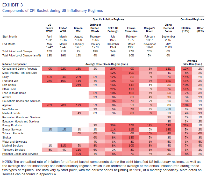
One concern when comparing inflationary episodes is whether each regime is driven by a different component of the basket and is therefore unique. Inflation-components data produced by the Bureau of Labor Statistics (BLS) suggest this is not the case. Exhibit 3 uses the US inflation periods defined in Exhibit 1 and tracks how various components of the CPI basket move. The available data give 125 regime-component pairs. Of these, 79 (63%) experience annualized inflation of 5% or more, our threshold for defining an inflationary regime. Looking at the averages, in 100% of instances, the basket component experiences higher rates of price rises during inflationary regimes than outside of them, and the rate is at least twice as high in 59% of instances.
FINANCIAL ASSETS
We now turn our attention to the performance of fi nancial assets during the eight US infl ationary regimes. In Exhibit 4, we tabulate the performance of a broad US equity index, the 10-year Treasury bond, and a 60–40 equity–bond portfolio. In the fi rst columns, we show the total returns during the eight infl ationary regimes, both in nominal terms (top panel) and real terms (bottom panel). At the top of the exhibit, we report some additional statistics that characterize the different periods. The next three columns show the annualized return over infl ationary, noninfl ationary, and all periods. The fi nal columns show the hit rate, defi ned as the proportion of regimes for which a given asset has yielded a positive return, and the t-statistic, which provides a heteroskedasticity-consistent test of whether returns are signifi cantly different in infl ationary and noninflationary times.
Starting with equities, we note that the nominal returns during infl ationary periods are zero on average, with negative returns in 50% of the infl ationary regimes. The real return averages -7% during infl ationary times, with negative returns in 75% of regimes. The real return is more relevant for most investors. These results are in line with the economic mechanisms presented earlier.
For the 10-year Treasury bond, the performance during high and rising inflation periods is also poor, which is not surprising for reasons already described. Although in nominal terms the average annualized return during infl ationary regimes is +3%, it is -5% in real terms. Consequently, the 60–40 equity–bond portfolio performs poorly during infl ationary regimes, with a -6% real annualized return.
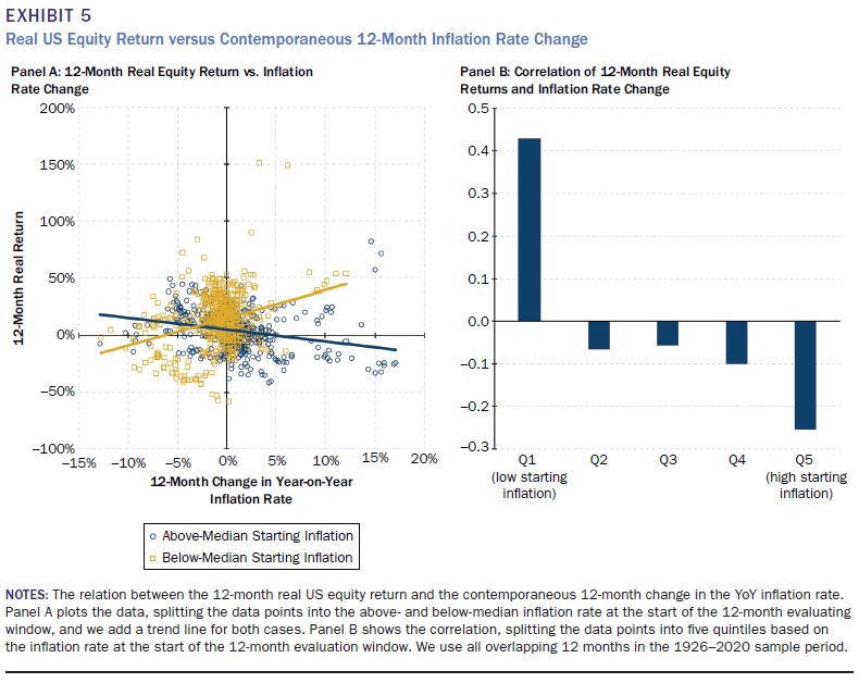
In Exhibit 5, we take a different approach, which serves as a robustness check to our regime analysis and allows us to explore how the equity response depends on the starting level of inflation.
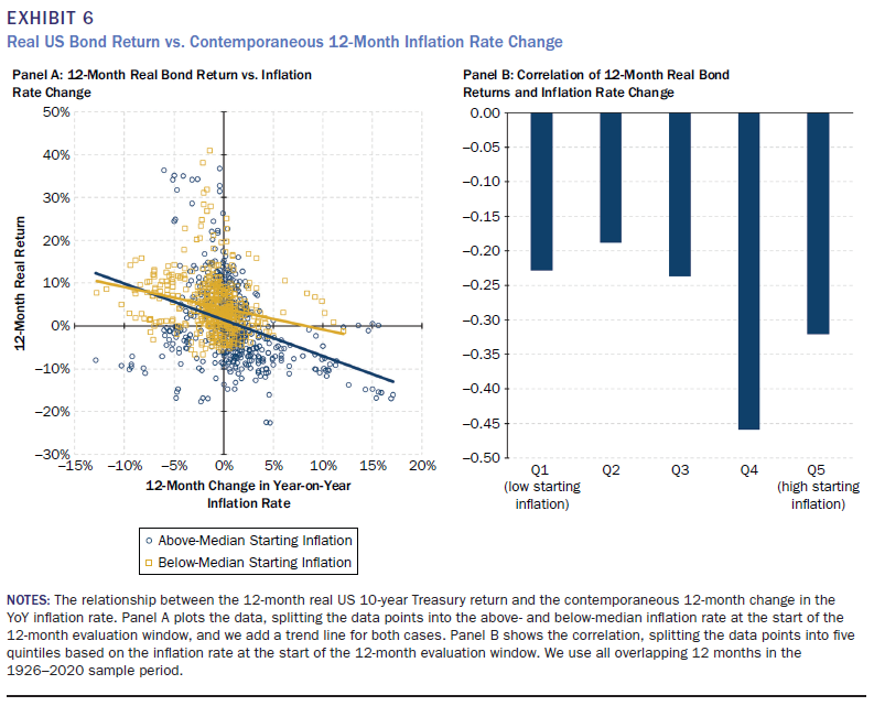
In the left panel, we show a scatter plot of the 12-month real return for equities versus the contemporaneous 12-month change in the YoY infl ation rate. We choose the 12-month change because it is more likely refl ective of long-term infl ation shocks. We separate instances in which the starting infl ation rate is below (yellow) and above (blue) the median level since 1926 (2.6%). The trend lines suggest that equities actually benefi t from rising infl ation if the starting level is below the median (risk of defl ation) but are hurt by rising infl ation if the starting level is above the median (increased risk of infl ation escalating). It is the latter effect that our regime analysis captures. A similar result can be gleaned from the right panel, in which we report the correlation between the 12-month real equity return and the contemporaneous 12-month change in the inflation rate for quintiles formed by the starting infl ation rate. Only in the lowest quintile (starting infl ation rate less than 1.0%) is the correlation positive at 0.4. In all other cases, there is a negative relationship between the real equity return and inflation changes, (monotonically) more so for higher starting levels of inflation.
In Exhibit 6, we repeat this exercise for real 10-year Treasury returns. The negative relation between bond returns and infl ation changes does not depend much on the starting level of inflation.
In Exhibit 7, we present the performance of different equity sectors. To conserve space, from now on, we will only report real returns. Only the energy sector has positive annualized real returns during infl ationary regimes. However, at +1%, it significantly lags the commodity it produces (see next section). Possible reasons for this include operational issues (e.g., the impact of wage infl ation or the fact that assets are often located in geopolitically turbulent regions) and the hedging strategies of the companies themselves, which may confound the transmission mechanism between commodity infl ation and higher profi ts for the producer.
Weak sectors include those with a high exposure to the individual consumer, such as durables (-15%) and retail (-9%). Technology (“business equipment” in the Fama and French 1997 categorization) is also -9%. Financials are weak because default risk dominates the benefi ts of possible rising rates and because there can be a lag between an infl ationary regime and central bank tightening. In Appendix C, we show a more granular split of US equity sectors.
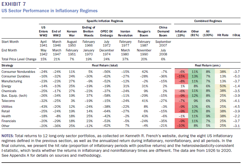
Exhibit 8 goes into more detail on fixed income. In terms of Treasury bonds, the higher the maturity, the greater the sensitivity to rising infl ation (which is typically paired with rising nominal yields). This is intuitive because higher maturity bonds have a higher duration. The annualized real return during inflationary regimes is -3% for the 2-year, -5% for the 10-year, and -8% for the 30-year bond.
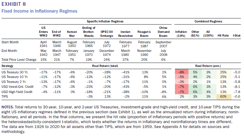
Neither investment-grade (IG) nor high-yield (HY) corporate bonds come close to protecting purchasing power, with both having a -7% real annualized return during infl ationary regimes. Both underperform government issuance at comparable tenor in the infl ationary regimes. The duration of the IG index ranges between six and eight years, whereas HY is between four and six years. This is less than the 10-year Treasury, which has tended to be between seven and nine. The shorter duration is not consistent with the weaker performance, and it is likely that recessionary fears
(and subsequent default risk) intensify through an infl ationary regime. The comparison makes clear that hedging IG and HY long positions with short government bond positions of similar duration did not provide infl ation protection in the past.
Finally, Exhibit 8 shows the performance of TIPS, which have coupon and principal payments that are indexed to the price level. The US Treasury only started to issue TIPS in 1997. However, data from a synthetic TIPS are available back to 1959 (Marshall 2020). The TIPS performance during the most recent fi ve infl ationary regimes is robust, with a 2% annualized real return, but not better than the real return in noninfl ationary times. It is noteworthy, however, that the starting TIPS yield in our infl ationary regimes was +2.4%, whereas it is currently -0.9%. The low yield
means that TIPS will be a very expensive infl ation hedge going forward (investors bear negative returns in noninflationary times).
HARD ASSETS
In this section, we consider hard assets: commodities, residential real estate, and collectibles. Such tangible assets may naturally adjust to changes in the overall price level and, in some cases, may explicitly be included in the basket of goods used to determine the infl ation rate (e.g., oil).
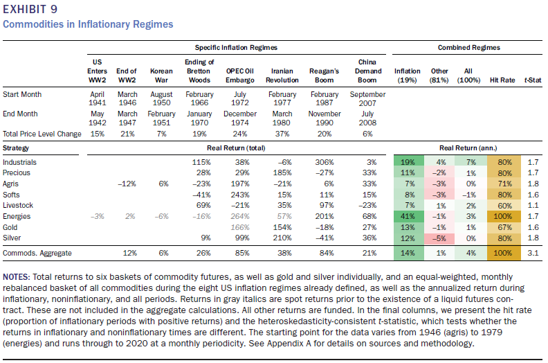
In Exhibit 9, we conduct the same exercise as in the previous exhibits with six commodity groupings, as well as gold and silver individually, and an aggregate commodity portfolio. Returns assume investment in commodity futures (plus a cash return to create a funded investment). All commodities have positive annualized real returns during infl ationary regimes. In fact, it is during noninfl ationary times that commodities tend to have a poorer performance of around +1% real. Thus, historically, commodities have not only been robust to rising infl ation but have also benefi tted from such an environment relative to normal times.
How does performance differ among commodity groups? Foodstuffs do least well, but still generate strongly positive real annual returns between 7% and 8%. The ending of the Bretton Woods episode is particularly weak for agris and softs (e.g., sugar, coffee, and cocoa). In a sense, this is idiosyncratic because it coincides with legislation across the 1960s designed to bring food prices down (e.g., the 1962–1963 repeal of the mandatory price support programs initiated in World War II). Precious and industrial metals do better, with returns of +11% and +19%, respectively. The stronger performance of the latter perhaps refl ects that, during infl ation, the substitute physical asset tendency is stronger than the substitute physical currency tendency. Energies lead by some margin at +41%.7
Some caution needs to be exercised in interpreting the commodity sector analysis. For example, with electric vehicle technology developing fast, it is likely that in the long term, oil and other brown economy fuels will lose the level of inflation performance they enjoyed in the past. However, over a shorter outlook, there are good reasons to think the historical pattern might hold: alternative fuels are yet to reach critical mass, and electric and hybrid vehicles made up just 4% of global automotive sales in 2020.8 In addition, there are many other reasons why inflation could have different effects on certain sectors: semiconductor shortages and the associated price hikes could affect the technology sector, and shortages of rare elements such as lithium may mean the inflationary impact on traditional commodities will differ from that indicated by the past.
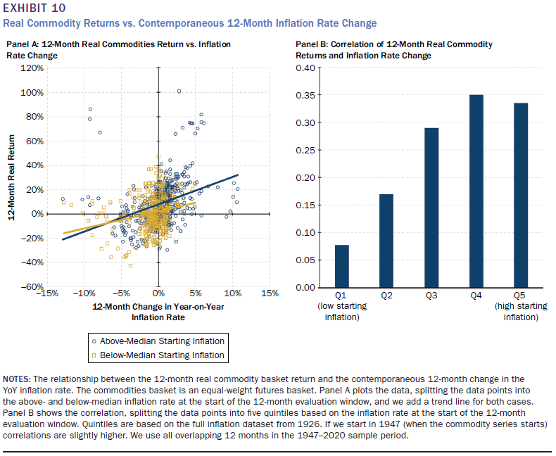
In Exhibit 10, we again take a different approach to evaluating aggregate commodity performance as a function of annual inflation rate changes, as we did in the previous section for equities and bonds. Consistent with those results, we see a positive relationship between the 12-month real return to the equally weighted commodity basket and the contemporaneous 12-month change in the inflation rate, irrespective of the starting level of inflation. From the right panel, we can see that the positive relation tends to be somewhat stronger when the inflation rate is in the top two quintiles.
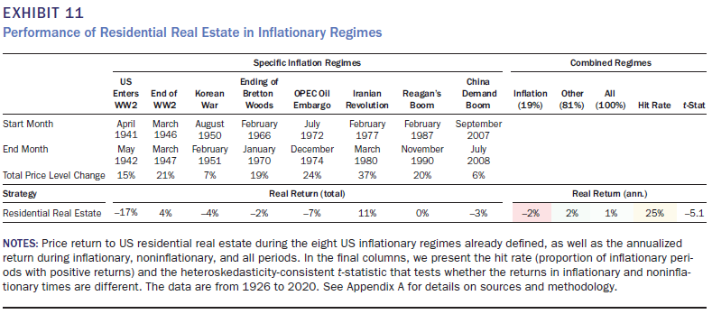
Next, we turn to residential property. In Exhibit 11, we see that US residential real estate has a small negative annualized real return of -2% during inflationary regimes, whereas it is +2% at other times. Thus, the asset does not seem to benefit from inflation in the same way commodities do; however, it could be argued that it is more robust than financial assets, with only a modest difference in the real returns between inflationary and other times. In Appendix B, we see that the UK real estate experience is similar to that in the United States, whereas for Japan (where our data capture the value of residential land rather than housing), the real return is higher during inflationary regimes than at other times.
Next, we consider collectibles, in particular art, wine, and stamps. In Exhibit 12, we show how these assets have performed through the eight US inflationary regimes. We find that collectibles have lived up to their reputation as a store of value in inflationary times. Real annual returns are positive during inflationary episodes for all three asset groups, with art at +7%, wine at +5%, and stamps +9%. Moreover, we notice a possible distinction between art and stamps (performance markedly improves in inflationary periods relative to normal times) and wine, which experiences lower but more consistent returns between normal and inflationary times.
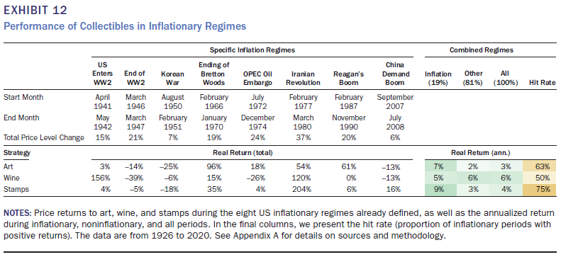
Collectibles are unlikely to be part of an institutional portfolio, given the small traded volumes. For instance, the global wine market turnover was $364 billion in 2019, according to Fortune Business Insights, of which collectible wine is a small sliver. To put that in context, the World Bank estimated global equity market turnover at $60 trillion in 2019.
ACTIVE STRATEGIES
So far, we have looked at passive investments in financial and hard assets. Now, we turn to active strategies. We first consider long–short stock factor portfolios. Second, we study trend strategies applied to futures and forwards.
For active strategies, implementation costs can be substantial. Therefore, we incorporate estimated costs, based on our live experience trading similar portfolios, which capture the combined effect of transaction, slippage, funding, and short-selling costs. The estimates are at the maximum of the range set forth by Harvey et al. (2019): 2.0% and 0.8% per annum for stock factor and future trend strategies, respectively. See Appendix A for further discussion on the costs of implementation.
In Exhibit 13, we show the performance of some well-known factor strategies through the eight US infl ationary regimes. Smaller companies perform poorly in infl ationary regimes. In real terms, the return for being long small size and short large size is -4% a year in infl ationary periods, compared to +1% in normal times. The factor is positive in just two of the eight episodes. This fi ts with intuition. The costs of infl ation will have some economies of scale benefi t. Take, for example, “shoe-leather costs,” meaning the extra effort that companies have to make when the value of cash is more volatile—making more trips to the bank and wearing out their shoes being the analogy (Fischer and Modigliani 1978). Larger companies are more suited to reacting to these conditions, given that they are more likely to have the necessary infrastructure to make such adaptations seamlessly.
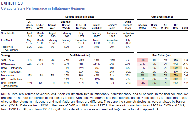
The profitability and value factors roughly hold their own during inflationary periods (-1% real return). The value performance might be surprisingly weak to some, given that higher-duration growth stocks are often assumed to be adversely sensitive to unexpected infl ation as discount rates increase. Still, it is worth saying that value long–short is still much more infl ation robust than the long-only fi nancial assets discussed previously.
Cross-sectional equity momentum historically performs well, with real inflation regime returns of +8% on average and a 75% hit rate across the eight episodes; however, we are somewhat cautious about the result, given the low t-statistic. In addition, the performance is highly sensitive to the dating of our regimes. For example, January 1975 was a very negative month for cross-sectional momentum, and our infl ationary regime stops in December 1974. Equally, late 2008 through early 2009 was catastrophic for momentum, and our infl ationary period ends in July 2008.
We also look at quality and low-beta premiums, using portfolios as formulated by Asness, Frazzini, and Pedersen (2019) and Frazzini and Pedersen (2014) (QMJ and BAB, respectively, in Exhibit 13). Although quality holds up well in the inflation regimes, low beta is weak, with a real annual average return of -3% and a hit rate of 25%. The duration effect may be prevalent here, given that low beta is often a play on long-term stable cash flows (e.g., non-CPI-linked utilities).
Some caution needs to be exercised in comparing these dynamic factor returns to long-only equity. These active strategies generally have low or even negative betas with the market. For example, over the full sample, the value factor has a beta of 0.2 and the low-beta factor has a beta of 0.1. The average returns are approximately the alpha of the strategy.
Next, we follow the methodology of Hamill, Rattray, and Van Hemert (2016) and Harvey, Rattray, and Van Hemert (2021) and construct a time-series momentum (trend) strategy applied to liquid futures and forwards. The strategy has a 10% ex ante annualized volatility target, and the weights to historical lags in the trend definition are chosen such that it best approximates the BTOP50 trend-following index returns.
In Exhibit 14, we observe that the annualized real return during infl ationary regimes is positive for each of the fi ve trend strategies, covering the four asset classes plus the all-asset version. For bonds and commodities, the real returns are positive during each of the individual inflationary regimes. This seems intuitive because bonds and commodities have a very clear exposure to infl ation (suffering and benefi tting from rising infl ation, respectively). Furthermore, for the bonds-and-commodities trend, the performance in rising infl ationary periods is much higher than during other periods. The all-asset class trend also performs relatively well during rising inflation periods. This is consistent with Baltussen, Swinkels, and Van Vliet (2020) who fi nd a positive exposure
of bond and commodity trend performance to changes in inflation expectations.
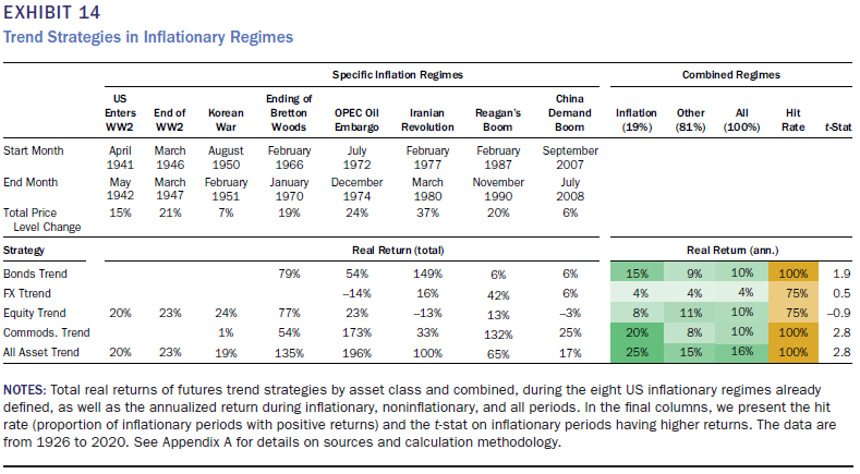
The active strategies provide some advantages. Although the trend-following strategies perform better than the equity factors, it is important to realize that the trend strategies have limited capacity, whereas the main equity factors have robust capacity. With that in mind, having a -1% real return for a value strategy, or a 3% average return for a quality strategy, does not look that bad. The equity factors do not experience the large negative returns that passive equity and fi xed-income investments experience during inflation shocks.
INTERNATIONAL INFLATION
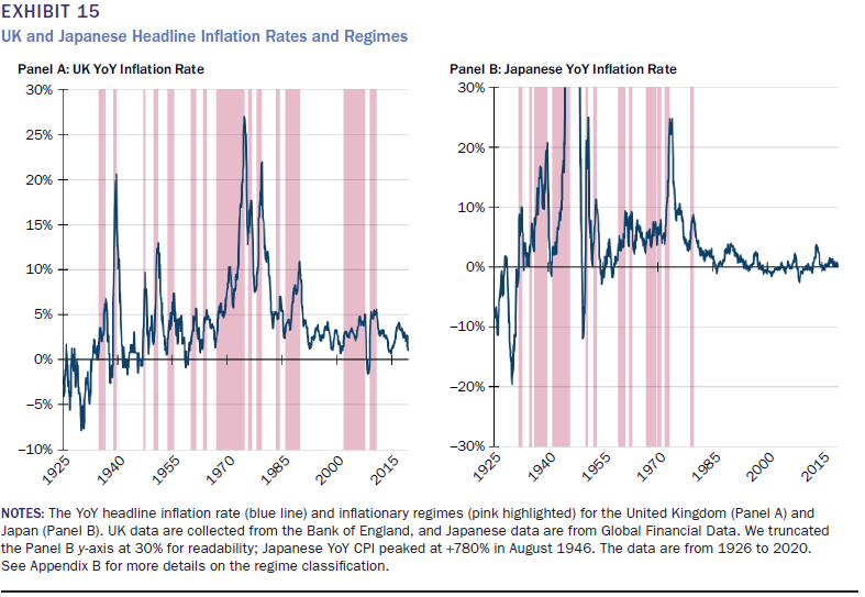
We perform an analysis for the United Kingdom and Japan similar to that we have done for the United States. We defi ne infl ationary regimes using the same method (i.e., when infl ation is accelerating above 5%, as already described) but based on local data. This results in the regimes presented in Exhibit 15. In Appendix B, we detail how a variety of local assets performed in the infl ationary periods for these countries, similar to the analysis in Exhibit 4 for the United States.
In Exhibit 16, we show a comparison of asset performance across all three nations. We note that performance is always from the vantage point of a specific country (base currency), which matters for realized infl ation correction. For active strategies, implemented with futures contracts, the base currency also matters for the interest earned on any unencumbered cash, just like investment
funds often have different currency share classes. We report the annualized real performance during the different regimes for the three countries and, in the final columns of the exhibit, split the sample period in terms of how many countries are in an inflationary regime.
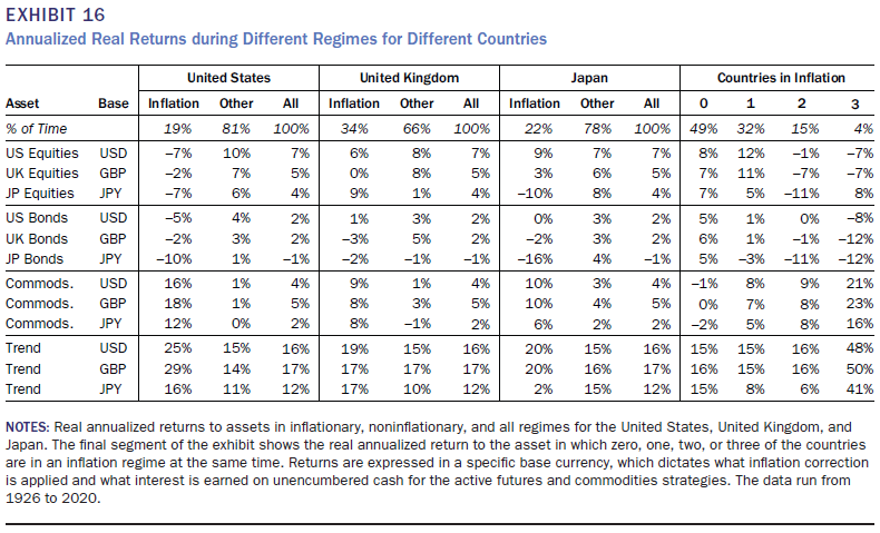
Equities tend to perform worst during their own country’s inflationary periods. US equities, for instance, achieve +6% and +9% real annualized return in UK and Japanese inflationary periods, compared to -7% in US regimes. The results also suggest benefits to international diversifi cation. For example, taking the UK perspective, US and Japanese equities generate +6% and +9% real annualized returns during UK inflation regimes, respectively.9 Importantly, equities work well when none of the three countries has high and rising infl ation (49% of the time) or when one of the three has it (32% of the time). Equities really only struggle when two or more countries are suffering. This is consistent with a global bout of infl ation being very negative for equity markets.
Bonds clearly perform the worst during their own country’s inflationary periods.
Commodities perform well during the inflationary periods of any one of these three countries. The effect is strongest during US inflationary regimes (running at a 15-percentage-point differential between infl ation and other regimes, compared to 8 for the United Kingdom and 7 for Japan). Commodities perform particularly well when all three countries are in an inflationary regime, which is about 4% of the months.
The all-asset trend strategy discussed in the previous section performs best during US inflationary periods, when the differential with normal times is 10 percentage points (+25% versus +15%). A possible driver here is US global economic leadership, both in terms of fundamentals and market prices, giving it fi rst-mover advantage as trends develop. Also, the trend strategy performs particularly well when all countries are in the inflationary regime.
STRUCTURAL CHANGE AND THE RISE OF CRYPTOCURRENCIES
As with any historical analysis, we are faced with the usual question: Is this time different? For example, the infl ation surge in the early 1970s was infl uenced by an exogenous event: the OPEC oil embargo. At the time, the US economy was highly dependent on that source of oil. Today is different because the United States is not as dependent on foreign oil sources. Moreover , although electric vehicles do not have critical mass today, such technological change in the future may make it much less likely that a surge in oil prices would have the same infl ationary effect. Hence,
caution needs to be exercised in interpreting the data. Indeed, this is precisely why most of our analysis focuses on regime behavior. Looking at averages over all regimes could be misleading because of one infl uential regime. For example, Erb and Harvey (2013) showed that gold’s seeming ability to hedge unexpected infl ation is driven by a single observation: 1979.
Other factors need to be carefully weighted given the structural evolution of the US economy. In the 1950s and 1960s, the United States was a manufacturing economy. Today, only 11% of GDP is driven by manufacturing.10 The nature of companies has changed. Much of the capital deployed is not physical but intangible, including trade secrets, proprietary software, patented and unpatented research and development, client relationships, and legal rights. These may be more resilient to inflation.
Finally, we are in the midst of another technological disruption in the form of cryptocurrencies, including bitcoin.11 Bitcoin is not controlled by any centralized authority—it is the result of a computer program that algorithmically increases the supply until it caps out at 21 million coins in 2140. This money supply rule induces algorithmic scarcity. This scarcity has some similarities to the scarcity of gold, given the limited amount of newly mined gold that comes to market each year.
Some have advocated for the inclusion of bitcoin into a diversified portfolio as an inflation protection asset. However, caution is warranted given that bitcoin is untested, with only eight years of quality data—over a period that that lacks a single inflationary regime. Moreover, bitcoin is five times more volatile than the S&P 500 or gold. This high volatility could lead to bitcoin being an unreliable hedge. Indeed, Erb and Harvey (2013) argued gold is an unreliable hedge over the short term because of its volatility.
Aside from this, there is evidence the price moves in bitcoin are not independent of economic events. Although, theoretically, bitcoin should have a zero inflation beta and zero market beta, reality is different. For example, in March of 2020 at the height of the COVID-19 crisis, investors began to reduce risk. The stock market dropped 34%, gold dropped 12%, and bitcoin plummeted 53% as investors poured money into safe-haven US Treasuries. As it became evident that the outlook was not as grim as first thought, investors returned to risky assets, with the stock market reaching
an all-time high, gold reaching its third-highest value in history, and bitcoin surging more than 800% (in the 12 months following its March 2020 trough). This suggests that bitcoin is a speculative asset and has a positive beta against the US market. Our analysis shows that unexpected high inflation is negatively related to US equity returns. The correlation of US equity and bitcoin returns suggests that bitcoin may not deliver positive real returns in periods of unexpected inflation.
CONCLUSIONS
Even if one forecasts a rate of inflation in the 2%–3% range over the next few years, it is likely that that forecast has a larger confidence interval than the same forecast at the end of 2019. Given the unprecedented monetary and fiscal interventions, most agree that inflation risk has increased. As such, it is time that portfolio managers review their asset positioning in the face of this heightened risk.
Our article is not about forecasting whether inflation will surge. We provide some evidence as to what may happen to the performance of a wide range of asset classes and active strategies if inflation does surge. Our analysis spans nearly a century. The long sample is particularly important because inflation spikes in developed economies have been rare in the past 30 years.
Our analysis takes two approaches. The first is the inflation beta approach in which an asset or strategy’s returns are correlated with unexpected inflation. An asset with a negative unexpected inflation beta provides a hedge—on average. The second approach focuses on specific regimes in which inflation has risen from a moderate level and crossed the 5% threshold. The advantage of this approach is that asset performance can be scrutinized in each regime. The inflation beta approach, in contrast, is just the average across all regimes.
Some of our analysis reaffirms what we already know. For example, Treasury bonds do poorly when inflation surges. Commodities, often being a source of inflation, do well. However, we offer additional insights. Commodities, for example, are a diverse set of assets, and their inflation-hedging properties depend on the individual commodity. Most importantly, we show that unexpected inflation is very bad news for equity investors.
We also examine a number of active strategies. Our results suggest that trendbased strategies focusing on equity, bonds, foreign exchange, and commodities have strong hit rates during the eight inflation episodes and provide an impressive level of protection. We consider a range of equity portfolios and find that popular factors such as value provide some benefit during inflationary times, as we define them. Although the average benefit is small (e.g., 3% real returns for a quality strategy to -1% for the value strategy), these factor portfolios perform far better than passive investments in stocks or bonds. The equity factors also have the extra advantage of high capacity.
1 These periods occurred during World War I and World War II. In 1918 and 1919, the deficit was 12% and 17%, respectively. In the 1942–1945 period, the annual defi cits were 12%, 27%, 21%, and 21%.
2 For example, early attempts to study the impact of unexpected inflation on asset returns include work by Fama and Schwert (1977), Kaul (1987), Fama (1981), Gultekin (1983), Beckers (1991), Lee (1992), Boudoukh and Richardson (1993), Ferson and Harvey (1993, 1994), Sharpe (1999), and Ang (2014).
3 In Exhibit 1, a negative inflection in real economic growth immediately follows five of eight US inflation regimes.
4 The United Kingdom introduced index-linked government bonds in 1981.
5 Indeed, it can be argued that 2% has been associated with price stability since the Reserve Bank of New Zealand pioneered central bank inflation targeting in the late 1980s.
6 The fourth decile of the distribution of US YoY inflation since 1926 is 2%. The eighth decile is 5%.
7 Erb and Harvey (2006) analyzed the inflation-hedging ability of a broader set of commodities, and Erb and Harvey (2013) analyzed the inflation-hedging performance of gold over long horizons. They
concluded that gold is too volatile to be a reliable inflation hedge and the performance since 1975 was largely driven by a single year, 1979, when gold dramatically appreciated in value.
8 Data from EV-Volumes.com.
9 This is perhaps one of the drivers behind the large international equity allocations run by some of the major UK pension funds coming out of the inflationary 1970s and 1980s. We do note that for
international diversification, exchange rate effects still need to be accounted for. Converted into GBP, the real annualized returns during UK inflationary regimes are 4% and 9% for US and Japanese equities.
APPENDIX A
FURTHER SOURCES AND CALCULATION METHODOLOGY
Inflation Measurements
For the United States, we use the BLS headline CPI index, as reported by Bloomberg. The components of inflation shown in Exhibit 3 are from the same source. In the early part of the history, some components report only quarterly or annually, and we therefore forward-fill the indexes where there are gaps.
Performance Statistics
For each of the asset performance exhibits, we show the regimes relevant to the country in question. For each regime, we show the real total return to the asset across the full time for which that regime endures (in case of Exhibits 4, B1, and B2, we also show the nominal returns). We also detail the length of the regime and the extent to which the headline CPI basket rose through it.
We then aggregate the data by showing the compound annual growth rate (CAGR) across all the regimes (8 in the United States, 14 in the United Kingdom, and 12 in Japan). If we do not have data for an asset over all of the regimes, we calculate the CAGR for the regimes that we have. Similarly, we calculate the CAGR for the asset in all other months (i.e., in which it was not within an inflationary regime) and then for the combined total.
After the aggregate returns, we present the hit rate, which is the percentage of inflation regimes in which the real return to the asset was positive (similarly for the nominal return in the case of Exhibits 4, B1, and B2). Finally, we calculate the heteroskedasticity- consistent t-statistic on a regression of the monthly returns to the asset on a constant plus a dummy variable that switches between 1 (in an inflationary regime) and 0 (not in an inflationary regime).
US Equities and Bonds
For US equities, we use Robert Shiller’s data for the S&P 500 total return history. For US 10-year Treasury bonds, we use Global Financial Data’s total return index. The 60–40 portfolio consists of a 60% S&P 500 and 40% US 10-year Treasury bond investment (capital weighted), rebalanced monthly. All returns to equities and bonds are assumed to be physical, cash-settled transactions.
US Fixed Income
Data for US Treasury nominal bonds of all three maturities are from Global Financial Data. Both the IG and HY indexes are calculated by Man Group based on data from Morgan Stanley Research. We take the IG spread and the BBB spread as a proxy for HY prior to 1980, and maturity data as reported by Morgan Stanley. We assume the indexes were issued at par in January 1921 and that coupons are paid semi-annually to deduce the modified duration. We then take default rates collated by Moody’s and assume a 40% recovery rate to calculate the total return.
The historical TIPS index is constructed by Goldman Sachs (Marshall 2020). To transform into a TIPS TR index, we use 10-year nominal yields to calculate the Macaulay duration, assuming a par rate, and then the estimated real yield to calculate the modified duration. To calculate the inflation accrual, we lag historical CPI by three months.
Commodities
Nominal returns are funded—in other words, the return of the contract plus the risk-free rate as reported by Kenneth French’s website. The real returns are the funded returns, minus inflation. The strategies take whichever futures contract is most liquid within the Man-AHL database. This is not always the first but will be in the early part of the curve. Groupings are as follows: industrials = copper; precious = gold, silver, and platinum; agris = wheat, corn, and soybeans; softs = cocoa, cotton, coffee, and sugar; livestock = cattle and hogs; and energies = Brent, WTI, and heating oil. Returns are equally weighted averages, month by month. Where one commodity in the group is not available, the average of the others is taken. The commodity aggregate category is a month-by-month, equally weighted average of all commodity groups. All returns are in US dollars. Gold spot returns are from the World Gold Council website.
Real Estate
US residential real estate data are from the Case–Shiller US home price index. In the early part of the series, the data are quarterly, and we linearly interpolate the missing values to make monthly data.
Collectibles
We focus on three long-term price series in particular: those for art, wine, and stamps. Goetzmann, Renneboog, and Spaenjers (2011) constructed an annual art price index from 1756–2007 using repeat-sales regression, based on sales pairs (of the same work). Dimson, Rousseau, and Spaenjers (2013) constructed a wine price index for the five Bordeaux Premier Grand Cru Classé chateaus from 1900–2012 using auction prices. Dimson and Spaenjers (2011) constructed an index for stamps from 1899–2008 using the Stanley Gibbons Stamp Catalogue covering 127 collectible stamps. Data are compiled in Credit Suisse’s Asset Returns Yearbook. These data are real, and we transform them to nominal using the long-term GDP deflator calculated in the Bank of England’s Millennium of Macroeconomic Data dataset. The series are annual, and we linearly interpolate them to get monthly values to match up with our regimes.
Active Equity Factors
Nominal returns are funded—in other words, we used the return of the Fama and French long–short factor plus the risk-free rate as reported on Kenneth French’s website. The real returns are the funded return (which adds the risk-free return), minus inflation. We assume 2% annual trading costs. The different factors are formed as a dollar-neutral portfolio that is long stocks that score high on the pertinent metric and short those that score low. The SMB factor is based on market capitalization; the HML factor uses the book-to-price ratio; the RMW factor orders stocks on EBT margin; the CMA factor uses the annual change in total assets; and momentum is based on the past 12-month return, skipping the most recent month.
The last two factors we look at are QMJ and BAB. These are taken from the work of Asness, Frazzini, and Pedersen (2019) and Frazzini and Pedersen (2014). Quality in QMJ is defined as a combination of profi tability (captured through a variety of profit and margin measures per unit of book value), growth (trailing fi ve-year growth in profits), and safety (market beta, volatility of profi ts, fi nancial leverage, and credit risk). Beta in the BAB strategy uses the capital asset pricing model.
It is worth giving a bit more detail on how we arrived at the 2% fi gure for annual trading costs. This is a simplification because active strategies such as cross-sectional momentum have much higher turnover than strategies like value. Partly this is just a matter of experience of the costs we feel when trading similar strategies. However, a similar result can be arrived at via the following:
Total costs = Dividend withholding tax + Slippage + Financing
Assume a dividend withholding tax of 30% and a yield of 2% (average US level), which gives 0.6% for the fi rst term. Given a holding period of three months and an average slippage of 6 bps, the cost would be
12m/3m× 2(Round trip trades) × 2(Gross book size) × 0.06% = 1.0%
We think 0.4% per annum is a reasonable expectation for fi nancing, so we get
0.6%(Dividend withholding tax) + 1.0%(Slippage) + 0.4%(Financing) = 2.0%
Trend
We follow the methodology of Hamill, Rattray, and Van Hemert (2016) and Harvey, Rattray, and Van Hemert (2021) and construct a time-series momentum (trend) strategy applied to liquid futures and forwards (or proxies) across assets, but we extend the data back further than their original work. For equities, we have data for Japan, the United Kingdom, the United States, Italy, Australia, and France from the 1926 start of our sample period. Other markets enter as they become available. For bonds, we have US bonds (different tenors) available since 1926, whereas most European bonds are included from 1950, some years after the dust of the second world war had settled. In commodities, we have soybeans, corn, and wheat starting between 1940 and 1950. Currencies still only start after the end of Bretton Woods in 1973. We assume annual transaction costs of 0.8%.
APPENDIX B
UNITED KINGDOM AND JAPAN
As discussed earlier, we have defi ned high and rising inflationary regimes for the United Kingdom and Japan using the same method we applied to the United States. We use the Retail Price Index (RPI) for the United Kingdom and the Nationwide Consumer Price Index (CPI) for Japan. There are differences in the basket weights of the three headline infl ation measures chosen, as would be expected in three regions with different consumption patterns. Shelter makes up 32% of the US CPI, 27% of the UK RPI, and 21% of the Japan CPI, as at September 2020. The US CPI is 60% services and 40% goods, whereas the other two are both broadly equally weighted in these categories. These differences are considered of secondary importance, however, when set against the requirement that the measure be widely disseminated and in the broadest use. The regimes that this approach yields are as we have already shown in Exhibit 15.
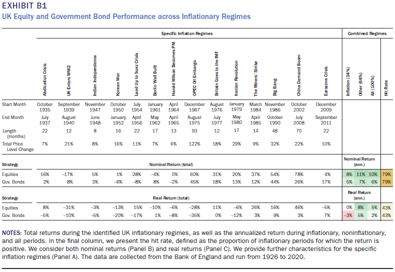
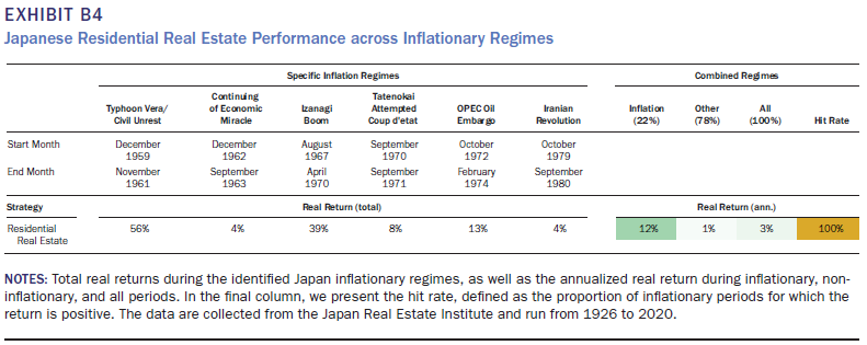
In Exhibits B1 and B2, we show the nominal and real returns for equities and nominal bonds in the United Kingdom and Japan, as we did in Exhibit 4 for the United States. The nominal returns are expressed in local currency (British pound and Japanese yen), and real returns are computed by adjusting for the local realized inflation. Results are broadly in line with the evidence for the United States, as presented before, in that both equities and government bonds have negative real returns, on average, during inflation regimes.
It is noted that UK equities do somewhat better than US stocks. In real terms, they are flat (fractionally negative) across the 14 regimes, with a 43% positive hit rate. As a reminder, the United States does -7% with a 25% hit rate. Possibly there is a currency effect here. In 1926, when our data start, the pound traded just below $5. Sterling depreciated fairly consistently to present-day levels below $2, but these depreciations were often particularly intense around infl ationary regimes, as would be expected. It may be that such moves were advantageous to the foreign-currency earnings of British stocks, which have always been proportionately significant. Possibly this provided some ballast for the performance of these securities.
Japan’s inflationary regime in World War II also bears mention as the one example of hyperinflation within our dataset. Between December 1941 and August 1946, Japan experienced a 1,432% rise in the general price level. Clearly, it is reductio ad absurdum, and hyperinflation is a very remote probability in the West today; however, it is still interesting that in this instance even diversified equity investors would have lost 95% of their purchasing power.
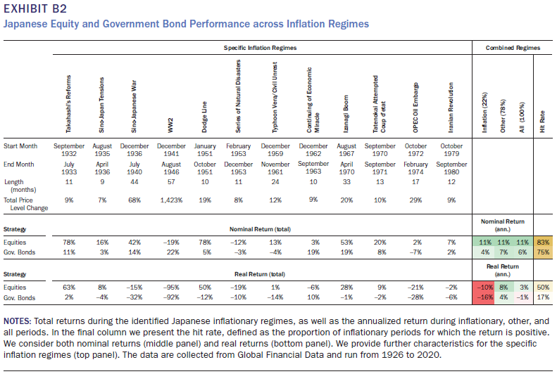
In Exhibit B3, we show the return to UK residential property. Real returns are positive, indicating some infl ation protection, but low and weaker than in normal regimes.
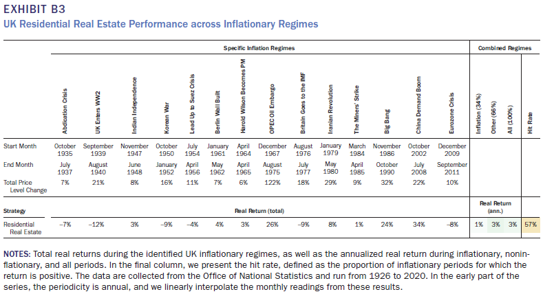
In Exhibit B4, we show the return to Japanese residential land, for which we have better data than for actual housing. Interestingly, Japan shows very strong returns to real estate, in particular contrast to the United States, with a real CAGR of +12% and a perfect hit rate. Clearly these regimes take one through Japan’s legendary real estate bubble. Indeed, at the peak in 1986, Tokyo real estate was changing hands at $139,000 per square foot, by which reckoning, it is often said, the Imperial Palace was worth more than the entire land value of California. Given these kind of historic extremes (and the crash that followed), we are hesitant to read too much into these results.
APPENDIX C
MORE GRANULAR EQUITY SECTORS
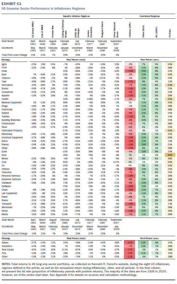
In Exhibit C1 we present real returns to sectors at a granular level. This supports the previous discussion around Exhibit 7 that no non-commodity sector provides meaningful inflation protection. Medical equipment is the only counterpoint, returning +1% real on average across the eight regimes. Gold miners are the strongest sector on +7%, outpacing other commodity producers. Longer duration sectors such as software (-20% real annualized) are particularly weak.
ACKNOWLEDGMENTS
We thank Tarek Abou Zeid, Ed Cole, Luke Ellis, Antoine Forterre, Carl Hamill, Soren Fryland Moller, Andrea Mondelci, Sandy Rattray, Graham Robertson, Matthew Sargaison, and Dan Taylor.
REFERENCES
Ang, A. 2014. Asset Management: A Systematic Approach to Factor Investing. Oxford: Oxford University Press.
Asness, C., A. Frazzini, and L. H. Pedersen. 2019. “Quality Minus Junk.” Review of Accounting Studies 24: 34–112.
Baltussen, G., L. Swinkels, and P. Van Vliet. 2020. “Global Factor Premiums.” Journal of Financial Economics, forthcoming.
Beckers, S. E. 1991. “Stocks, Bonds, and Infl ation in World Markets: Implications for Pension Fund Investment.” The Journal of Fixed Income 1 (3): 18–30.
Boudoukh, J., and M. Richardson. 1993. “Stock Returns and Infl ation: A Long-Horizon Perspective.” The American Economic Review 83 (5): 1346–1355.
Dimson, E., P. L. Rousseau, and C. Spaenjers. 2013. “The Price of Wine.” Journal of Financial Economics 118 (2): 431–449.
Dimson, E., and C. Spaenjers. 2011. “Ex Post: The Investment Performance of Collectible Stamps.” Journal of Financial Economics 100 (2): 443–458.
Erb, C. B., and C. R. Harvey. 2006. “The Tactical and Strategic Value of Commodity Futures.” Financial Analysts Journal 62 (2): 69–97.
——. 2013. “The Golden Dilemma.” Financial Analysts Journal 69 (4): 10–42.
Fama, E. F. 1981. “Stock Returns, Real Activity, Inflation, and Money.” The American Economic Review 71 (4): 545–565.
Fama, E. F., and K. R. French. 1997. “Industry Costs of Equity.” Journal of Financial Economics 43 (2): 153–193.
Fama, E. F., and G. W. Schwert. 1977. “Asset Returns and Inflation.” Journal of Financial Economics 5 (2): 115–146.
Ferson, W. E., and C. R. Harvey. 1993. “The Risk and Predictability of International Equity Returns.” The Review of Financial Studies 6 (3): 527–566.
——. 1994. “Sources of Risk and Expected Returns in Global Equity Markets.” Journal of Bankingand Finance 18 (4): 775–803.
Frazzini, A., and L. H. Pedersen. 2014. “Betting against Beta.” Journal of Financial Economics 111 (1): 1–25.
Goetzmann, W. N., L. Renneboog, and C. Spaenjers. 2011. “Art and Money.” American Economic Review: Papers & Proceedings 101 (3): 222–226.
Gultekin, B. 1983. “Stock Market Returns and Inflation: Evidence from Other Countries.” The Journal of Finance 38 (1): 49–65.
Hamill, C., S. Rattray, and O. Van Hemert. 2016. “Trend Following: Equity and Bond Crisis Alpha.” Working paper, SSRN.
Harvey, C. R., E. Hoyle, S. Rattray, M. Sargaison, D. Taylor, and O. Van Hemert. 2019. “The Best of Strategies for the Worst of Times: Can Portfolios Be Crisis Proofed?” The Journal of Portfolio
Management 45 (5): 7–28.
Harvey, C. R., A. Ramachandran, and J. Santoro. 2021. DeFi and the Future of Finance. Hoboken, NJ: John Wiley and Sons (forthcoming).
Harvey, C. R., S. Rattray, and O. Van Hemert. 2021. Strategic Risk Management. Hoboken, NJ: John Wiley and Sons.
Kaul, G. 1987. “Stock Returns and Inflation: The Role of the Monetary Sector.” Journal of Financial Economics 18 (2): 253–276.
Lee, B. 1992. “Causal Relations among Stock Returns, Interest Rates, Real Activity and Inflation.” The Journal of Finance 47 (4): 1591–1603.
Marshall, W. 2020. “A Backcast History of Traded Inflation.” Goldman Sachs.
Sharpe, S. “Stock Prices, Expected Returns, and Inflation.” Working paper, Federal Reserve Board, 1999
This information herein is being provided by GAMA Investimentos (“Distributor”), as the distributor of the website. The content of this document contains proprietary information about Man Investments AG (“Man”) . Neither part of this document nor the proprietary information of Man here may be (i) copied, photocopied or duplicated in any way by any means or (ii) distributed without Man’s prior written consent. Important disclosures are included throughout this documenand should be used for analysis. This document is not intended to be comprehensive or to contain all the information that the recipient may wish when analyzing Man and / or their respective managed or future managed products This material cannot be used as the basis for any investment decision. The recipient must rely exclusively on the constitutive documents of the any product and its own independent analysis. Although Gama and their affiliates believe that all information contained herein is accurate, neither makes any representations or guarantees as to the conclusion or needs of this information.
This information may contain forecasts statements that involve risks and uncertainties; actual results may differ materially from any expectations, projections or forecasts made or inferred in such forecasts statements. Therefore, recipients are cautioned not to place undue reliance on these forecasts statements. Projections and / or future values of unrealized investments will depend, among other factors, on future operating results, the value of assets and market conditions at the time of disposal, legal and contractual restrictions on transfer that may limit liquidity, any transaction costs and timing and form of sale, which may differ from the assumptions and circumstances on which current perspectives are based, and many of which are difficult to predict. Past performance is not indicative of future results. (if not okay to remove, please just remove reference to Man Fund).
No investment vehicle managed by Man is an affiliate of, Gama , any administrator, placement agent or controlling person for Gama or any of their respective affiliates.

