
Link para o artigo original: https://www.man.com/insights/regimes-systematic-models-power-of-prediction


Regimes, Systematic Models and the Power of Prediction
March 24, 2025
Discovering we’re in an economic regime after the fact risks missing vital information for adapting investment processes. How can we employ systematic methods to identify economic regimes and use them to predict returns?
Introduction
Not that long ago, we hardly heard the word ‘regime’ mentioned in the markets. Then came the post-COVID inflationary spike, and suddenly they were ‘flavour of the month’. In fact, we’ve long thought that regimes – specific market environments characterised by distinct macroeconomic, financial and geopolitical conditions over a set time period – offer a useful perspective on performance and risk that is unfettered from the days and months of the calendar.
We began this paper having already spent a good deal of time working on regimes, both within Man Numeric’s Macroscope models1 and in the Fire and Ice framework2 that has guided our approach to inflation modelling. We wanted to use these different approaches to identification and implementation to think about regimes from the bottom up, constructing a simple model that characterises markets by their similarity or difference when compared to historical periods.
The existing research on regimes is useful in constructing a balanced portfolio that is robust against different regimes. By contrast, the aim of this paper is to provide a point-in-time metric for timing investments. It does so by proposing a systematic approach to regime selection (a ‘Regime Model’).
The main contribution of our paper is methodological. However, we do apply our Regime Model to six popular long-short equity factors. We look at historical factor returns and go long a factor if the historical return subsequent to observing the regime at the investment date is positive, and short otherwise.
We document a positive relation between the returns on this type of strategy, and similarity. Indeed, the least similar historical dates do the worst in terms of performance. The alpha of being long the most similar and short the least similar is a statistically significant three standard deviations from zero. Exhibit 1 suggests that the strategy is also a consistent performer.
Exhibit 1. Long similarity and short dissimilarity
Yearly returns from regime model implementation at 15 volatility
Problems loading this infographic? – Please click here
Source: Man Group internal data as at 2025. For a full list of data sources, please see Exhibit 2.
In writing this paper, we have reviewed and leant on much of the existing research on regimes. For example, Kaya et al. (2010)3 offer a useful early model, recognising in their paper that emphasising current conditions rather than preset regime characteristics is a more useful way of considering a market landscape which is in constant evolutionary flux. However, unlike the prior studies, which either impose discrete regime classifications or rely on statistical models with predefined transitions, our approach allows for a more flexible definition of regimes by directly measuring historical similarity across multiple economic variables.
We should say here that this paper is not intended to be either complex or comprehensive. The driving idea behind our research was to establish a framework and model that were both intuitive and flexible and could therefore be used as the basis for further research.
The Regime Model methodology
The user of our Regime Model needs to specify a set of economic variables, and in this paper, we consider a constellation of seven variables. We transform these variables to look at annual changes and compute a z-score. Then, variable by variable, we investigate the past and identify regimes that are similar.4 Looking at every historical date, we aggregate the distances at each date across our seven variables. We refer to the aggregated similarity score as the ‘Global Score’. Those historical dates with the smallest aggregate distances are our definition of similar regimes. Once we have established similar dates in the past for a particular asset, we look at subsequent returns. Importantly, once the historical regimes are established, we can apply this method to any asset class.
Our Regime Model has several advantages. First, the method is systematic, in that the regime classifications are automatic. Second, the method can easily be applied to a much larger set of economic variables. Third, our method is simple, relying only on z-scores.
That said, in any systematic model, choices need to be made. In our method, the economic state variables need to be chosen (which itself induces look-ahead bias). Second, there is a choice as to how to represent the variable (e.g., what horizon for rate of change?). Third, we need to agree the degree of similarity. Fourth, we need to decide on the length of the observation period after the similar historical regime. Finally, how should we weight the economic variables?
Economic state variables
Identification of variables
We use the seven economic state variables detailed in Exhibit 2:5
Exhibit 2. Economic state variables and sources
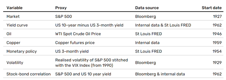
Our chosen economic state variables are all financial variables that embed macroeconomic information. Again, this is our choice, and the user of our method could add a range of different macroeconomic variables.
For each variable, we take a 12-month change and then normalise it by computing the z-score over a rolling 10 years, capped to be within minus three and three.6 Next, we compute an adjustment similar to a z-score, whereby we divide the one-year difference by the standard deviation of the rolling one-year differences, computed over 10 years. We finish by winsorizing at three to remove outliers, thereby creating the transformed economic state variables.
Descriptive statistics
We are now able to assess the properties of the transformed series of variables. We do this both individually (autocorrelations) and across series (correlations). As expected, the autocorrelation largely vanishes by 12 months. The cross-correlations of the variables are generally low (with the highest positive correlation occurring between the two commodities – oil and copper – at 0.36). The low average absolute cross-correlations suggest that the seven economic variables contain independent information. This provides some diversification, and, in a way, these variables deliver a non-parametric basis for a signal (i.e. it doesn’t contain pre-defined assumptions, is flexible and any conclusions are only derived from the data itself).
Determining similar dates
We now apply our distance-based similarity metric. This runs on an iterative basis, whereby each month we compute the Euclidean distance – the distance ‘as the crow flies’ between two points – between each historical month and the month in question. We are then able to aggregate across our variables, to obtain one Global Score.7 Historical months with smaller similarity scores are the most similar to today.8
Similarity in action: Three crisis periods
To illustrate how our Regime Model works, we choose three different situations of stress: the Global Financial Crisis (GFC), COVID-19, and the 2022 inflation surge. For specific months, we examine the full history and pick the 15% most similar months (i.e., the 15% of months with the lowest values of the Global Score). We exclude the last three years (36 observations) when measuring similarity, as this helps us to avoid loading up on momentum.
Referring to the GFC, Exhibit 3 considers the global score as of January 2009. The time series measures the similarity between all historical dates and January 2009. The most similar dates have the lowest values and include all observed recessions. To preview our trading strategy, we would take a long position in an asset in February 2009 that exhibits positive returns after historically similar regimes.
Exhibit 3. Historical similarity to January 2009 during the Global Financial Crisis
Problems loading this infographic? – Please click here
Source: Man Group internal data as at 2025. For a full list of data sources, please see Exhibit 2.
Secondly, the COVID-19 period was a period of a large drawdown and a sharp recovery. This time series reveals no obvious visual patterns, and this is likely because the COVID-19 crisis was so unique (at least in the last 100 years).
Finally, we look at the inflation surge of 2022, particularly August 2022. In contrast to COVID-19, there is plenty of experience with inflation within our sample. Our model shows this month most similar to the inflation period following the Iranian revolution of 1977-1980.9
Assessing the predictive power of the Regime Model
We illustrate the efficacy of our methodology on six long-short stock factors: using the Fama-French five research factors (Market, Size, Value, Profitability and Investment) plus the 12-month Momentum factor.
Exhibit 4 shows the performance of investing in the six factors using the 20% most similar historical dates (quintile one). We are long a factor if the average of returns after the most similar dates was positive, and short if it was negative. So, we are using the Regime Model to “time” the factors. The performance shown is when aggregating across the six timed factors on an equally weighted basis. We repeat this exercise for the other quintiles, and so quintile five utilises the 20% most dissimilar dates. On the left-hand chart in Exhibit 4, we have included the performance of quintile one and quintile five (alongside a representative long-only model (LO model) which serves as a proxy for a traditional long-only portfolio). We have only included quintiles one and five because our analysis shows that, of the five quintiles, quintile one performs best and quintile five performs worst. While you can see that the LO model performs slightly better than quintile one over time, it brings with it significantly worse drawdowns during crisis periods.
Exhibit 4. Assessing the predictability using six long-short stock factors10

Source: Man Group internal data as at 2025. For a full list of data sources, please see Exhibit 2.
As factors tend to have positive returns on average, the timed portfolio is far more likely to be long a factor. Indeed, the first-quintile returns are 0.76 correlated to a static long-only portfolio, going long all six factors all the time. The other quintiles’ returns have a positive correlation to the long-only portfolio as well. This means we can create a less correlated ‘difference’ portfolio by going long the quintile-one portfolio and short the quintile-five portfolio (Exhibit 4, right-hand chart). This portfolio has an impressive 0.82 Sharpe ratio, while only being 0.37 correlated to the long-only portfolio. The alpha is significant, being three standard errors from zero.
The difference portfolio combines two elements: returns today that are most similar to returns subsequent to similar dates in the past and returns today that are most dissimilar to returns subsequent to past dissimilar dates.
Conclusion: Diversification via multiple variables
We present a systematic method to identify economic regimes. Our Regime Model assesses the similarity of any month to the history of a selection of economic time series. The user specifies the economic time series as well as the tolerance for similarity. The method is non-parametric, using simple z-scores to measure how similar a month is compared to each historical month. The user can specify many economic variables to achieve a type of diversification that is not possible with a single or even dual variable method.
We use our method to actively time six well-known factors. We aggregate all factors and find there is important information in the similarity. The strategy based on the most similar periods does well. We also find that in the anti-regime months (the most dissimilar), the performance is poor.
There are many research enhancements that are possible here. Currently, we equally weight all economic variables. One can imagine a dynamic weighting based on predictive performance. Further, we assess similarity with respect to particular months. If the investment horizon is longer than a month, it might be reasonable to look at similarity relative to a quarter or even longer. These and related ideas are for future research into economic regimes.
The authors would like to thank Alex Preston for his valuable comments.
1. See Views from the Floor 2001 Redux? Today’s Economy Shows Eerie Parallels to Post-Dot-Com Crash | Man Group for example.
2. See Fire, Then Ice | Man Group or 10 for 10: Themes for the Next Decade | Man Group.
3. Kaya, Hakan, Wai Lee, and Bobby Pornrojnangkool. “The Journal of Portfolio Management.” The Journal of Portfolio Management, vol. 36, no. 2, Winter 2010, pp. 94–105. DOI: 10.3905/JPM.2010.36.2.094.
4. Our measure of similarity is the squared distance of today’s value to each historical observation. For example, if the z-score today is 2.5, we look at historically similar times where the z-score is close to 2.5. If the value on a particular historical date was exactly 2.5, the squared distance would be zero.
5. These were selected after a systematic process to establish which variables were the most important driver of equity returns.
6. We use monthly data so that we can extend our history as far back as possible. For the correlation series we use a rolling three-year metric. We run this on daily data before converting to monthly.
7. The Euclidean distance, d, is defined by: dTi=vVxiv-xTv2 . On a selected month T, for every historical month i, we calculate a sum of squares of the V transformed variables. We do so by computing the absolute difference between the value of each variable at month i, xiv, and the value of each variable at month T, xT v. We sum across variables before taking the square root, to give us our similarity score, dT i, for every month up to month T.
8. This calculation must be done historically for every historical month. For example, if the variable has a score of 2.5 in December 2024, we calculate the distance between each historical month and 2.5. If the score was 2.1 in November 2024, we need to again calculate the difference between all historical months and the score of 2.1.
9. It also loads onto a few months from the 1966-1970 inflation period associated with the ending of the Bretton Woods, the OPEC oil embargo inflation period of 1972-1974 and Reagan’s boom between 1987 and 1990.
10. The performance of investing in six long-short stock factors (Market, Size, Value, Profitability, Investment, Momentum). For the quintile one portfolio, the direction taking in a factor is based on returns subsequent to the 20% most similar historical dates. The quintile five portfolio utilizes the 20% most dissimilar returns. The long-only portfolio is long all six factors throughout. Performance is shown for 1985-2024. Input data starts well before 1985 to allow for rolling-window calibrations.
This information herein is being provided by GAMA Investimentos (“Distributor”), as the distributor of the website. The content of this document contains proprietary information about Man Investments AG (“Man”) . Neither part of this document nor the proprietary information of Man here may be (i) copied, photocopied or duplicated in any way by any means or (ii) distributed without Man’s prior written consent. Important disclosures are included throughout this documenand should be used for analysis. This document is not intended to be comprehensive or to contain all the information that the recipient may wish when analyzing Man and / or their respective managed or future managed products This material cannot be used as the basis for any investment decision. The recipient must rely exclusively on the constitutive documents of the any product and its own independent analysis. Although Gama and their affiliates believe that all information contained herein is accurate, neither makes any representations or guarantees as to the conclusion or needs of this information.
This information may contain forecasts statements that involve risks and uncertainties; actual results may differ materially from any expectations, projections or forecasts made or inferred in such forecasts statements. Therefore, recipients are cautioned not to place undue reliance on these forecasts statements. Projections and / or future values of unrealized investments will depend, among other factors, on future operating results, the value of assets and market conditions at the time of disposal, legal and contractual restrictions on transfer that may limit liquidity, any transaction costs and timing and form of sale, which may differ from the assumptions and circumstances on which current perspectives are based, and many of which are difficult to predict. Past performance is not indicative of future results. (if not okay to remove, please just remove reference to Man Fund).


